While working on latency control and reduction on a real-time multimedia application, I discovered that the first problem I had was the latency variations introduced by network conditions. The main challenge I had was estimating the network disorder only with an incoming RTP stream, without RTCP control and feedback packets. The following article describes the method used to estimate the network disorder and deduce an optimal buffer duration for the current conditions.
Background
Lets say we have an application that streams a multimedia (video and/or audio) real-time stream to a receiver. By real-time we mean that the content streamed may be interactive and can’t be send in advance to the receiver (like an audio/video call for instance).
Context
The source emits the stream over the network to the receiver. Usually the encoded content is split in small access units, encapsulated in RTP packets, sent over UDP. To simplify we’ll assume that the source only sends a video stream using RTP over UDP to the target.
The target receives the RTP packets on a random UDP port and obtains the packets through a socket, as usual. As RTP defines it, each packet has a timestamp that describes the presentation time of the access unit (see RFC3550 for more details on RTP). As an access unit might be bigger than the maximum RTP payload size, it might be split over multiple RTP packets. The method to do this depends on the codec, so avoid useless difficulties, we’ll consider that the receiver has a assembler that delivers each access unit reassembled with its presentation timestamp.
In the following paragraphs, we’ll consider the access units and their presentation timestamps before/after it enters/goes out the RTP/UDP transport layer. It is almost equivalent as working on RTP packets, so for the purpose of this article it is a reasonable assumption.
The problem: network and time reference
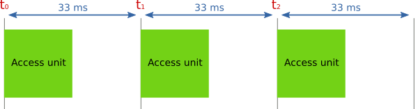
On emitter side, access units are produced on a regular basis. For a 30 frames per second video stream we usually have one access unit every 33 milliseconds (to be fair it depends on the codec). The illustration below shows a stream of access units emitted following a 33ms clock period (30 frames per second).
If the network was kind of perfect, we should receive exactly the same stream (with the same interval between access units) with a small delay due to the emission, transmission, reception and assembly operations.
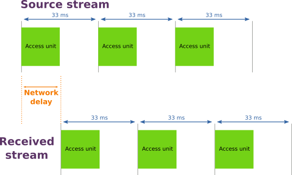
But in real life, the network delay is not a constant. There’s a constant part due to the incompressible processing and transmission delays, there is also a variable part due to network congestion. So the real result looks like the following illustration.
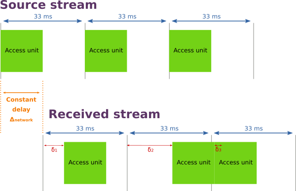
Each access unit is delivered on the receiver with a delay, regarding its original clock, that varies according to network conditions. The latency of an access unit can be represented by:
\Delta_{frame}(n) = \Delta_{network} + \delta_nNow let’s summarize the receiver situation:
- it receives an access unit stream with their presentation timestamp (to be precise an equivalent RTP stream),
- access unit are not delivered on a regular basis because the delivery depends on network conditions,
- network conditions are evolving over time,
- the only available time references are the access unit timestamp.
The challenge will be to find a way to estimate the required buffer duration to be able to play the access unit stream smoothly without being disturbed by network hazards.
Inter-arrival jitter as network conditions estimator
To estimate network congestion and then compute an adequate buffering duration, we need to find a indicator. Looking for some papers on the subject I found a RFC draft: Google Congestion Control Algorithm for Real-Time Communication. This algorithm deduces a Receiver Estimated Maximum Bitrate (REMB) using the inter-arrival jitter. Computing a bitrate is not exactly what we want to do but it uses only the incoming RTP packets and their timestamps to do the estimation.
Inter-arrival jitter
The timestamps associated to the frames are not enough to compute the overall latency of the stream. But thanks to them, we have a valuable information: the theorical delay between two frames. It is equivalent to the delay between two frames emissions from the source. The difference between timestamps T of frames n and n-1 is what we call the inter-departure time:
T(n) - T(n-1)
On the other hand, as a receiver, we can record the time of arrival for each frame and compute the difference between arrival timestamps t for frames n and n-1. This is what we call the inter-arrival time:
t(n) - t(n-1)
If we compare the inter-departure and the inter-arrival times we have an indicator of the network congestion: the inter-arrival jitter. In a formal way the inter-arrival jitter can be defined with the following formula:
J(n) = t(n) - t(n-1) - (T(n) - T(n-1))
A precise description of the inter-arrival time filter model is available in the RFC draft here.
Estimations
Observing the jitter is a good way to get information about network conditions because it represents the distance between the ideal situation (the departure delays) and the reality (the arrival delays) . The more the jitter is far from zero, the more the network is disturbed.
The first estimator we can compute is the average of the jitter. It provides an estimation of the network disorder over time, but to represent the “current” disorder correctly, it needs to be a sliding average. In Chromium implementation of GCC, an exponential moving average is used. It allows to keep the influence of the more recent jitter samples over a defined period while smoothing big variations.
\alpha \text{ is the moving average coefficient} \\
J(n) \text{ is the inter-arrival jitter for frame } n \\
J_{avg}(n) \text{ is the moving average for frame } n \\
J_{avg}(n) = \alpha * J(n) + (1 - \alpha) * J_{avg}(n-1)
The smoothing parameter α has to be chosen according to the use case and the implementation. If we’re playing a 30 frames per second stream, a value of 0.1 for α means the average applies applies overs 10 jitter values, so it takes into account the last 10 * 33ms = 330ms.
The average is a good start but a weak indicator because it is highly sensitive to variations and does not provide any information on the distribution of the jitter. To be more precise, we’re not interested in a buffer that satisfies the mean jitter but that takes into account most of the jitter of incoming frames. Don’t forget that our goal is to have a smooth playing experience!
We would like to have an indicator that allows us to estimate a buffer duration that smoothes the network impact for almost all frames. Saying this, it seems obvious we need a buffer duration with a confidence interval. If we compute the standard deviation σ from jitter samples, we can build a confidence interval around the mean jitter value that provides the correct buffering duration for 68% (average plus σ), 95% (average plus 2σ) or even 99.7% (average plus 3σ) and so on. To learn more on standard deviation and confidence interval, read here.
We can compute a moving variance over the jitter samples using the exponential average:
V(n) = \alpha * (J_{avg}(n) - J(n))^2 + (1 - \alpha) * V(n-1) And then the standard deviation for the last set of samples:
\sigma(n) = \sqrt{V(n)}Let’s take an example! After some seconds, the average jitter is 15 ms and the standard deviation 37 ms. If we consider using the 3σ confidence interval, the buffer duration calculation is:
D_{buf}(n) = J_{avg}(n) + 3 * \sigma(n) = 15 + 3 * 37 = 126 \text{ ms}Using this interval, it should cover 99.7% of the frame jitters. The buffer duration can be estimated regularly over the time to adjust the duration to the optimal value. Doing this, we are keeping the latency to the lowest value possible while preserving the stream quality.
Conclusion
Statistics over the inter-arrival jitter is the simpler way I found in the litterature to estimate a correct buffer duration. It provides a smooth playing experience while keeping the latency to the lowest possible level without breaking the quality. It requires very few inputs (only an incoming RTP stream with timestamps) to produce a reliable network quality indicator.
Acknowledgements
- Tristan Braud for helping me understand the concepts behind jitter measures and the statistics leading to buffer duration.
- Rémi Peuvergne for advices on the article content and the drawings.